More Usage Examples

Here we simulate multivariate autoregressive processes from papers in order to show how various directed connectivity measures work. See the papers for details.

import numpy as np
import matplotlib.pyplot as plt
from spectral_connectivity import Multitaper
from spectral_connectivity import Connectivity

from spectral_connectivity.simulate import simulate_MVAR


def plot_directional(time_series, sampling_frequency, time_halfbandwidth_product=2):
    m = Multitaper(
        time_series,
        sampling_frequency=sampling_frequency,
        time_halfbandwidth_product=time_halfbandwidth_product,
        start_time=0,
    )
    c = Connectivity(
        fourier_coefficients=m.fft(), frequencies=m.frequencies, time=m.time
    )

    measures = dict(
        pairwise_spectral_granger=c.pairwise_spectral_granger_prediction(),
        directed_transfer_function=c.directed_transfer_function(),
        partial_directed_coherence=c.partial_directed_coherence(),
        generalized_partial_directed_coherence=c.generalized_partial_directed_coherence(),
        direct_directed_transfer_function=c.direct_directed_transfer_function(),
    )

    n_signals = time_series.shape[-1]
    signal_ind2, signal_ind1 = np.meshgrid(np.arange(n_signals), np.arange(n_signals))

    fig, axes = plt.subplots(
        n_signals, n_signals, figsize=(n_signals * 3, n_signals * 3), sharex=True
    )
    for ind1, ind2, ax in zip(signal_ind1.ravel(), signal_ind2.ravel(), axes.ravel()):
        for measure_name, measure in measures.items():
            ax.plot(
                c.frequencies,
                measure[0, :, ind1, ind2],
                label=measure_name,
                linewidth=5,
                alpha=0.8,
            )
        ax.set_title("x{} → x{}".format(ind2 + 1, ind1 + 1), fontsize=15)
        ax.set_ylim((0, np.max([np.nanmax(np.stack(list(measures.values()))), 1.05])))

    axes[0, -1].legend()
    plt.tight_layout()

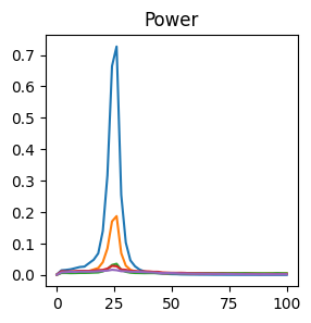
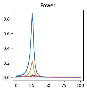
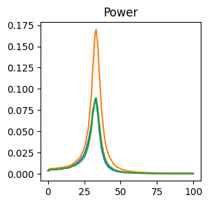
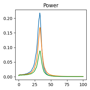
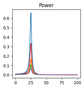
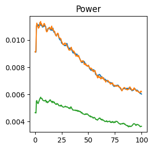
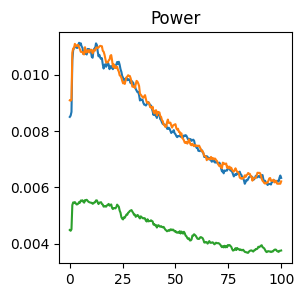
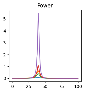
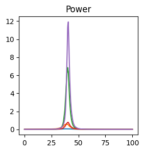
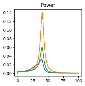
    fig, axes = plt.subplots(1, 1, figsize=(3, 3), sharex=True, sharey=True)
    axes.plot(c.frequencies, c.power().squeeze())
    plt.title("Power")

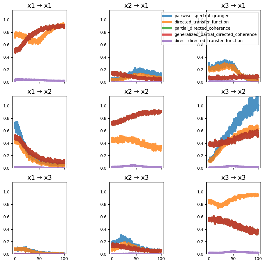
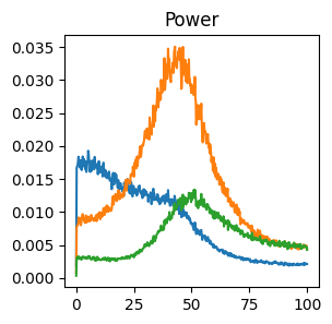
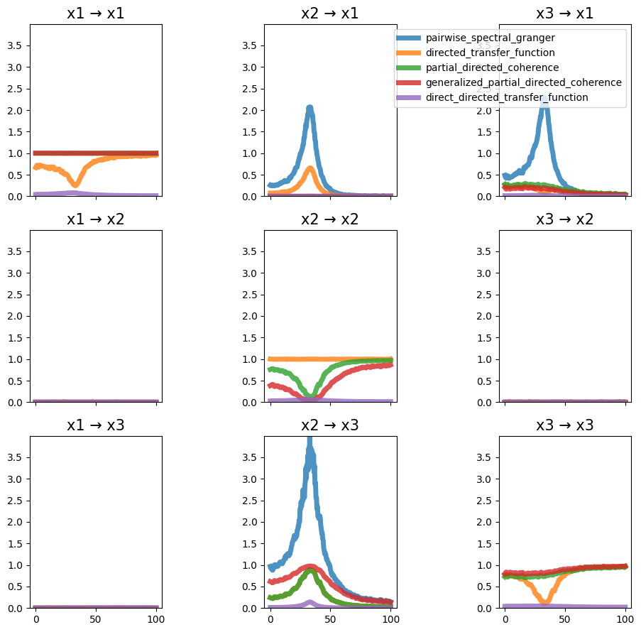
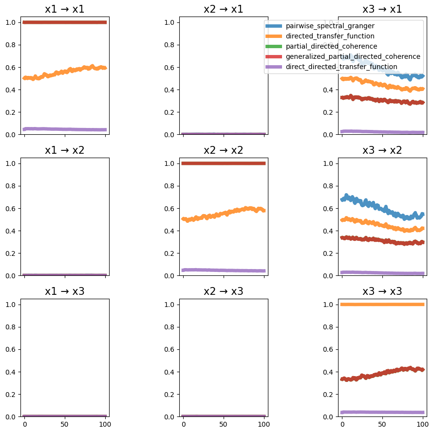
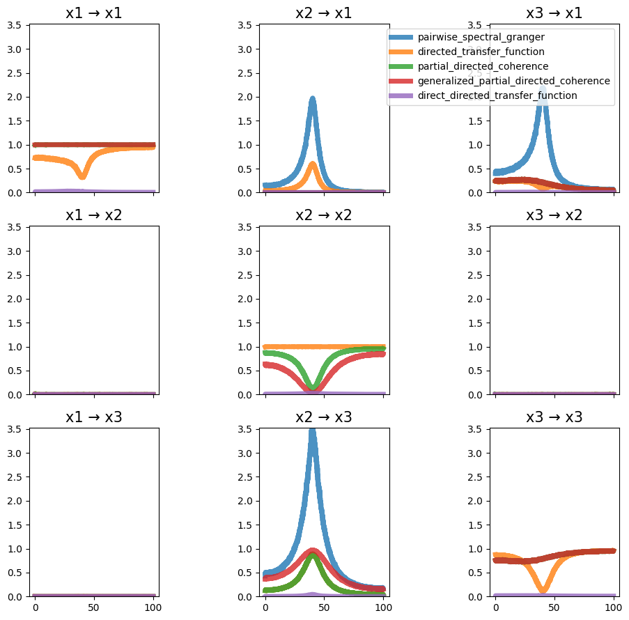
Baccala Example 2

Baccalá, L.A., and Sameshima, K. (2001). Partial directed coherence: a new concept in neural structure determination. Biological Cybernetics 84, 463–474.

\[x_1 = 0.5x_1(n-1) + 0.3x_2(n-1) + 0.4x_3(n-1) + w_1(n)\]

\[x_2 = -0.5x_1(n-1) + 0.3x_2(n-1) + 1.0x_3(n-1) + w_2(n)\]

\[x_3 = -0.3x_2(n-1) - 0.2x_3(n-1) + w_3(n)\]

def baccala_example2():
    """Baccalá, L.A., and Sameshima, K. (2001). Partial directed coherence:
    a new concept in neural structure determination. Biological
    Cybernetics 84, 463–474.
    """
    sampling_frequency = 200
    n_time_samples, n_lags, n_signals = 1000, 1, 3

    coefficients = np.array([[[0.5, 0.3, 0.4], [-0.5, 0.3, 1.0], [0.0, -0.3, -0.2]]])

    noise_covariance = np.eye(n_signals)

    return (
        simulate_MVAR(
            coefficients,
            noise_covariance=noise_covariance,
            n_time_samples=n_time_samples,
            n_trials=500,
            n_burnin_samples=500,
        ),
        sampling_frequency,
    )


plot_directional(*baccala_example2(), time_halfbandwidth_product=1)

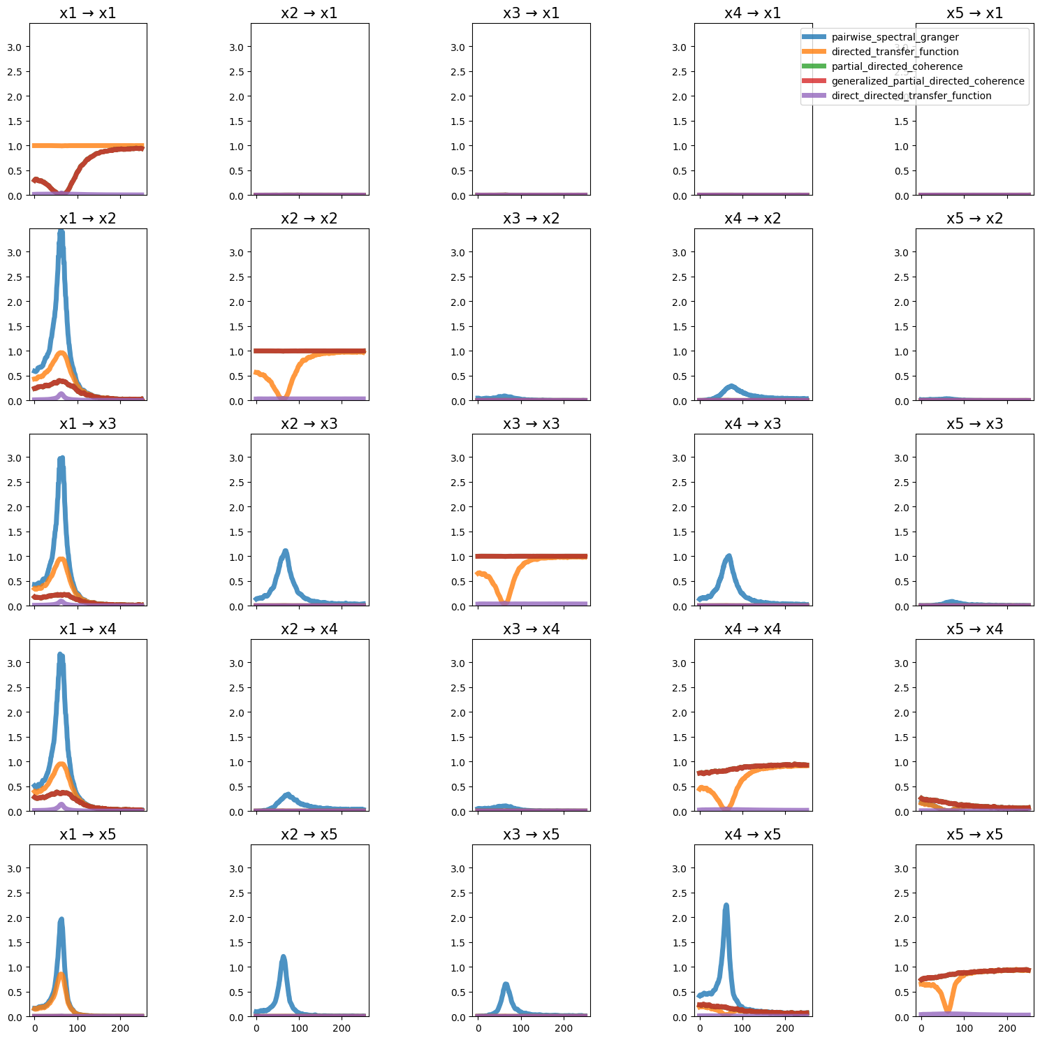
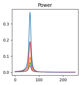
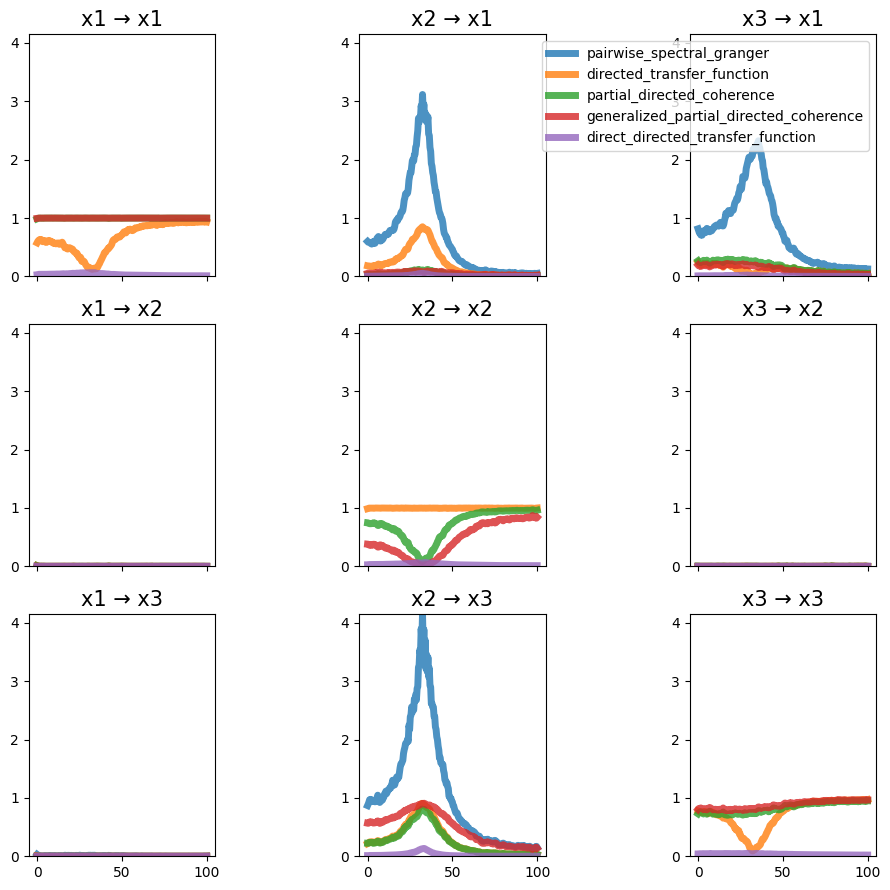
Baccala Example 3

Baccalá, L.A., and Sameshima, K. (2001). Partial directed coherence: a new concept in neural structure determination. Biological Cybernetics 84, 463–474.

def baccala_example3():
    """Baccalá, L.A., and Sameshima, K. (2001). Partial directed coherence:
    a new concept in neural structure determination. Biological
    Cybernetics 84, 463–474.
    """
    sampling_frequency = 500
    n_time_samples, n_lags, n_signals = 510, 3, 5
    coefficients = np.zeros((n_lags, n_signals, n_signals))

    coefficients[0, 0, 0] = 0.95 * np.sqrt(2)
    coefficients[1, 0, 0] = -0.9025

    coefficients[1, 1, 0] = 0.50
    coefficients[2, 2, 0] = -0.40

    coefficients[1, 3, 0] = -0.5
    coefficients[0, 3, 3] = 0.25 * np.sqrt(2)
    coefficients[0, 3, 4] = 0.25 * np.sqrt(2)

    coefficients[0, 4, 3] = -0.25 * np.sqrt(2)
    coefficients[0, 4, 4] = 0.25 * np.sqrt(2)

    noise_covariance = None

    return (
        simulate_MVAR(
            coefficients,
            noise_covariance=noise_covariance,
            n_time_samples=n_time_samples,
            n_trials=500,
            n_burnin_samples=500,
        ),
        sampling_frequency,
    )


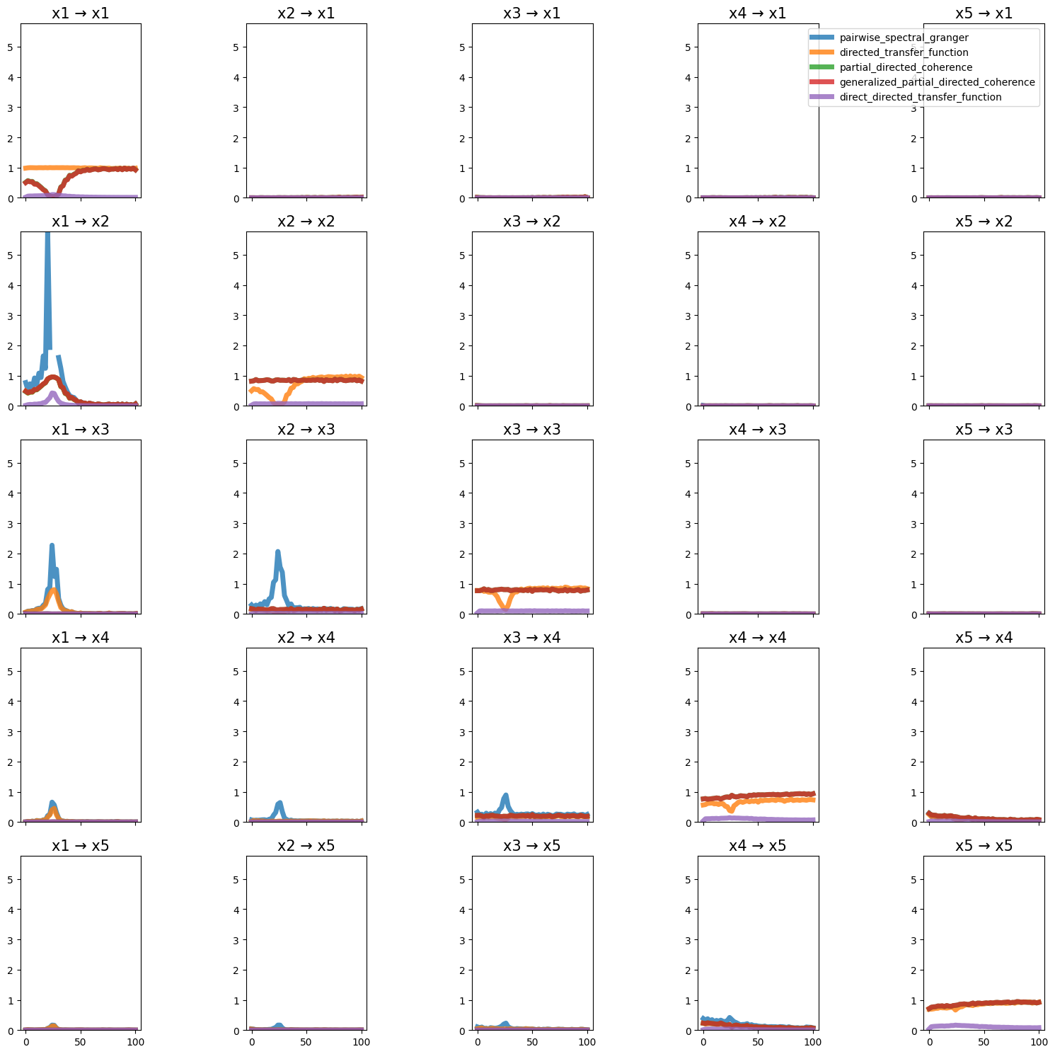
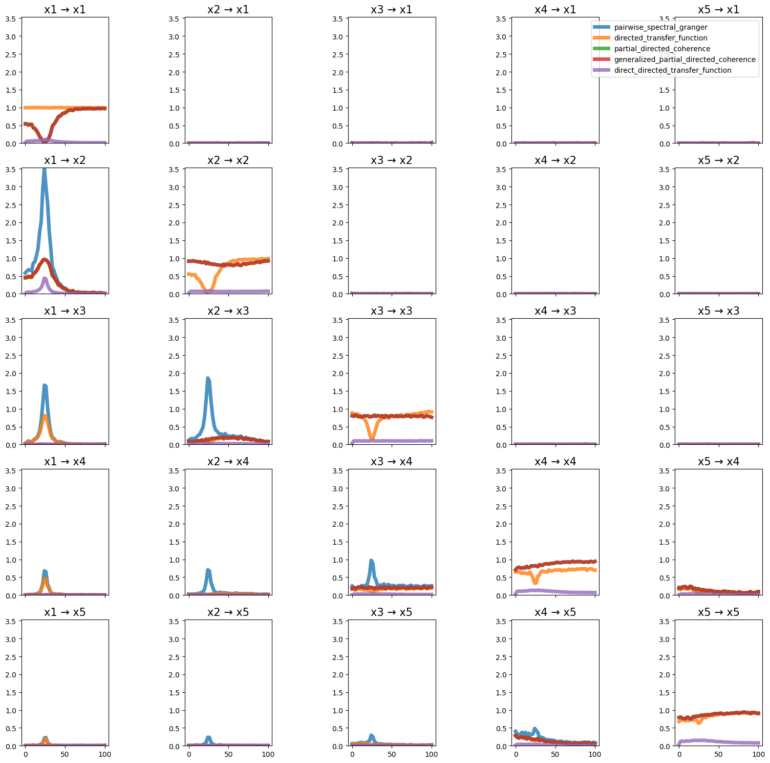
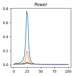
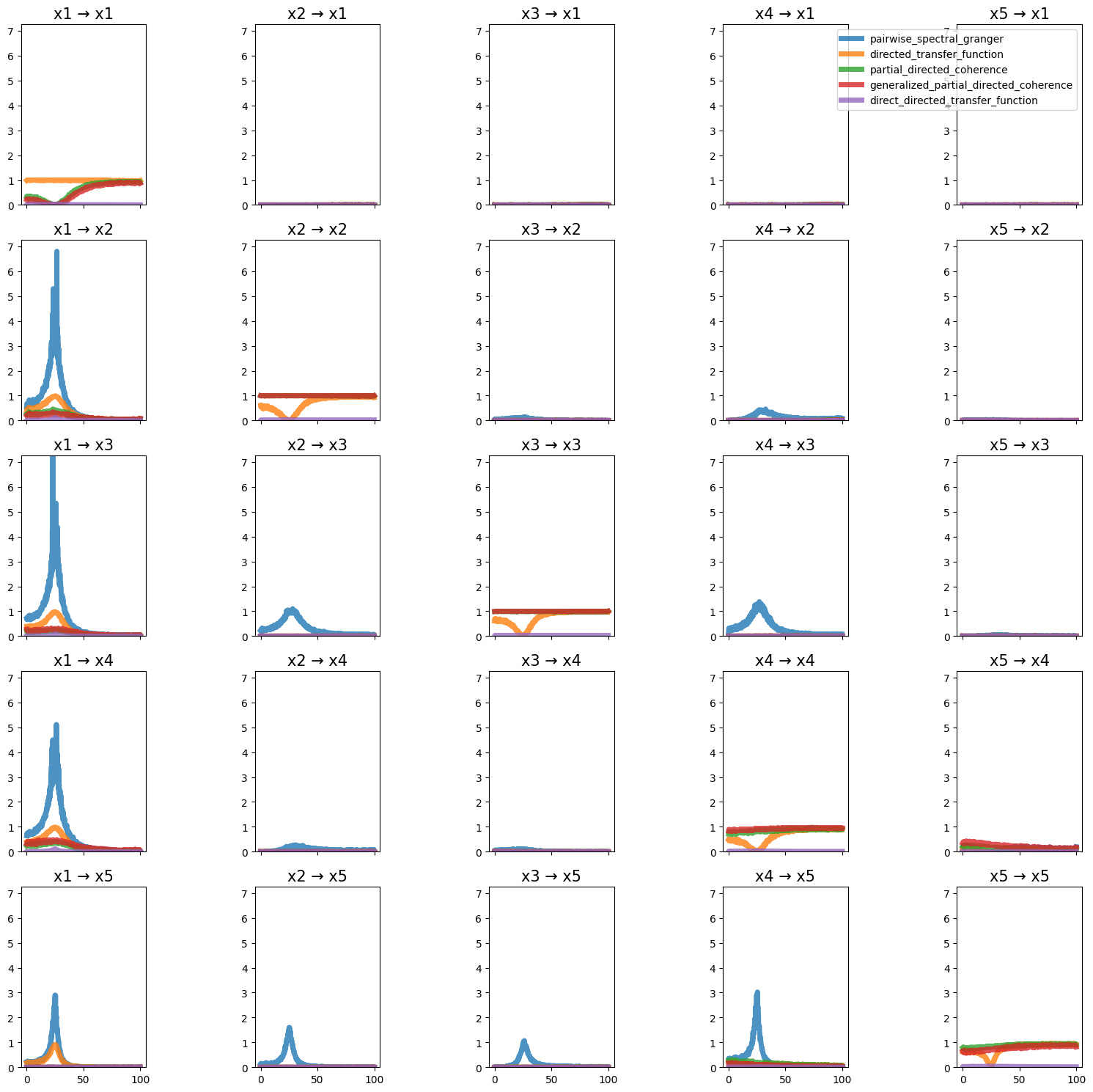
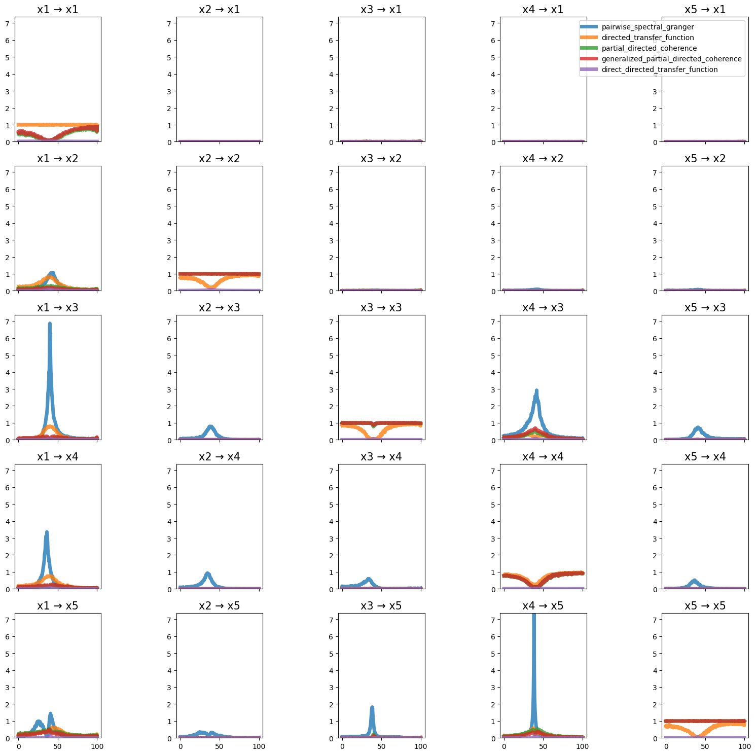
plot_directional(*baccala_example3(), time_halfbandwidth_product=3)

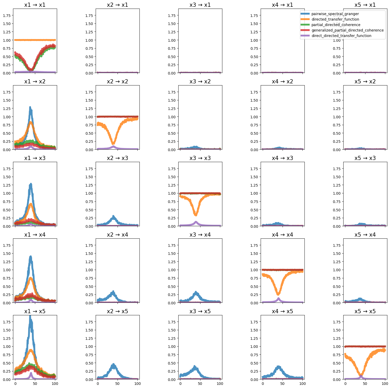
Baccala Example 4

Baccalá, L.A., and Sameshima, K. (2001). Partial directed coherence: a new concept in neural structure determination. Biological Cybernetics 84, 463–474.

def baccala_example4():
    """Baccalá, L.A., and Sameshima, K. (2001). Partial directed coherence:
    a new concept in neural structure determination. Biological
    Cybernetics 84, 463–474.
    """
    sampling_frequency = 200
    n_time_samples, n_lags, n_signals = 100, 2, 5
    coefficients = np.zeros((n_lags, n_signals, n_signals))

    coefficients[0, 0, 0] = 0.95 * np.sqrt(2)
    coefficients[1, 0, 0] = -0.9025
    coefficients[0, 1, 0] = -0.50
    coefficients[1, 2, 1] = 0.40
    coefficients[0, 3, 2] = -0.50
    coefficients[0, 3, 3] = 0.25 * np.sqrt(2)
    coefficients[0, 3, 4] = 0.25 * np.sqrt(2)
    coefficients[0, 4, 3] = -0.25 * np.sqrt(2)
    coefficients[0, 4, 4] = 0.25 * np.sqrt(2)

    noise_covariance = None

    return (
        simulate_MVAR(
            coefficients,
            noise_covariance=noise_covariance,
            n_time_samples=n_time_samples,
            n_trials=500,
            n_burnin_samples=500,
        ),
        sampling_frequency,
    )


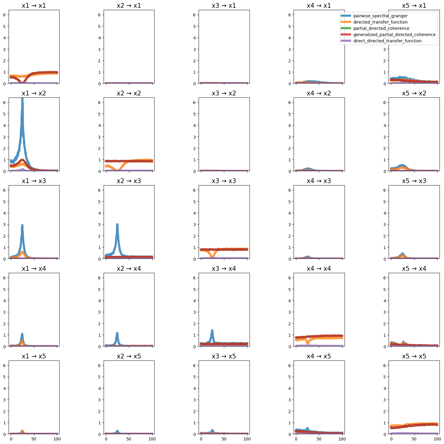
plot_directional(*baccala_example4(), time_halfbandwidth_product=1)

Baccala Example 5

Baccalá, L.A., and Sameshima, K. (2001). Partial directed coherence: a new concept in neural structure determination. Biological Cybernetics 84, 463–474.

def baccala_example5():
    """Baccalá, L.A., and Sameshima, K. (2001). Partial directed coherence:
    a new concept in neural structure determination. Biological
    Cybernetics 84, 463–474.
    """
    sampling_frequency = 200
    n_time_samples, n_lags, n_signals = 510, 2, 5
    coefficients = np.zeros((n_lags, n_signals, n_signals))

    coefficients[0, 0, 0] = 0.95 * np.sqrt(2)
    coefficients[1, 0, 0] = -0.9025
    coefficients[1, 0, 4] = 0.5
    coefficients[0, 1, 0] = -0.50
    coefficients[1, 2, 1] = 0.40
    coefficients[0, 3, 2] = -0.50
    coefficients[0, 3, 3] = 0.25 * np.sqrt(2)
    coefficients[0, 3, 4] = 0.25 * np.sqrt(2)
    coefficients[0, 4, 3] = -0.25 * np.sqrt(2)
    coefficients[0, 4, 4] = 0.25 * np.sqrt(2)

    noise_covariance = None

    return (
        simulate_MVAR(
            coefficients,
            noise_covariance=noise_covariance,
            n_time_samples=n_time_samples,
            n_trials=500,
            n_burnin_samples=500,
        ),
        sampling_frequency,
    )


plot_directional(*baccala_example5(), time_halfbandwidth_product=1)

Baccala Example 6

Baccalá, L.A., and Sameshima, K. (2001). Partial directed coherence: a new concept in neural structure determination. Biological Cybernetics 84, 463–474.

def baccala_example6():
    """Baccalá, L.A., and Sameshima, K. (2001). Partial directed coherence:
    a new concept in neural structure determination. Biological
    Cybernetics 84, 463–474.
    """
    sampling_frequency = 200
    n_time_samples, n_lags, n_signals = 100, 4, 5
    coefficients = np.zeros((n_lags, n_signals, n_signals))

    coefficients[0, 0, 0] = 0.95 * np.sqrt(2)
    coefficients[1, 0, 0] = -0.9025
    coefficients[0, 1, 0] = -0.50
    coefficients[3, 2, 1] = 0.10
    coefficients[1, 2, 1] = -0.40
    coefficients[0, 3, 2] = -0.50
    coefficients[0, 3, 3] = 0.25 * np.sqrt(2)
    coefficients[0, 3, 4] = 0.25 * np.sqrt(2)
    coefficients[0, 4, 3] = -0.25 * np.sqrt(2)
    coefficients[0, 4, 4] = 0.25 * np.sqrt(2)

    noise_covariance = None

    return (
        simulate_MVAR(
            coefficients,
            noise_covariance=noise_covariance,
            n_time_samples=n_time_samples,
            n_trials=500,
            n_burnin_samples=500,
        ),
        sampling_frequency,
    )


plot_directional(*baccala_example6(), time_halfbandwidth_product=1)

Ding Example 1

Ding, M., Chen, Y., and Bressler, S.L. (2006). 17 Granger causality: basic theory and application to neuroscience. Handbook of Time Series Analysis: Recent Theoretical Developments and Applications 437.

\[ x_1 = 0.9x_1(n-1) -0.5x_1(n-2) + w_1 \]

\[ x_2 = 0.8x_2(n-1) -0.5x_2(n-2) + 0.16x_1(n-1) -0.2x_1(n-2) + w_2 \]

def ding_example1():
    """Ding, M., Chen, Y., and Bressler, S.L. (2006). 17 Granger causality:
    basic theory and application to neuroscience. Handbook of Time Series
    Analysis: Recent Theoretical Developments and Applications 437.
    """
    sampling_frequency = 200
    n_time_samples, n_lags, n_signals = 1000, 2, 2
    coefficients = np.zeros((n_lags, n_signals, n_signals))

    coefficients[0, ...] = np.array([[0.90, 0.00], [0.16, 0.80]])
    coefficients[1, ...] = np.array([[-0.50, 0.00], [-0.20, -0.50]])

    noise_covariance = np.array([[1.0, 0.4], [0.4, 0.7]])

    return (
        simulate_MVAR(
            coefficients,
            noise_covariance=noise_covariance,
            n_time_samples=n_time_samples,
            n_trials=500,
            n_burnin_samples=500,
        ),
        sampling_frequency,
    )


plot_directional(*ding_example1(), time_halfbandwidth_product=3)

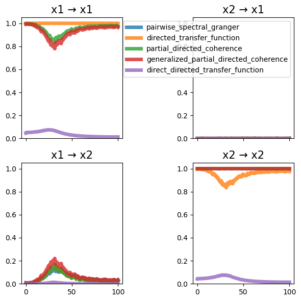
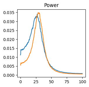
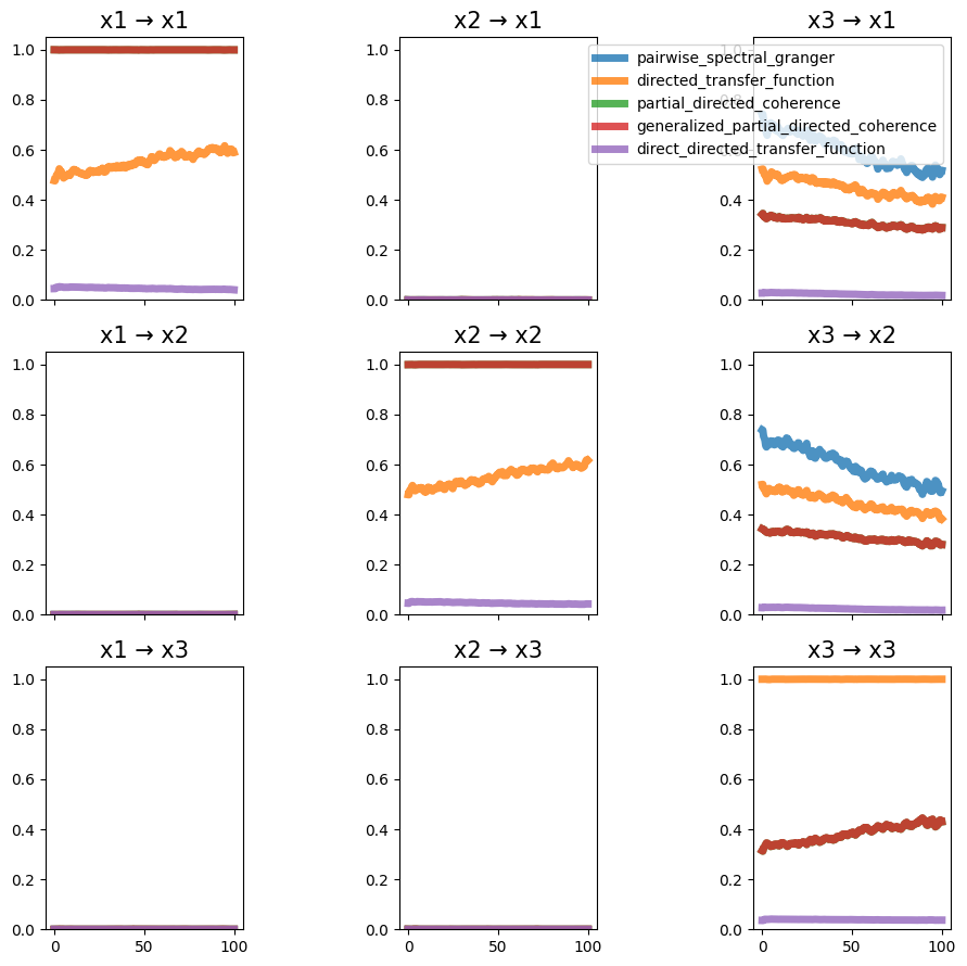
Ding Example 2a

Ding, M., Chen, Y., and Bressler, S.L. (2006). 17 Granger causality: basic theory and application to neuroscience. Handbook of Time Series Analysis: Recent Theoretical Developments and Applications 437.

\[ x_1 = 0.8x_1(n-1) - 0.5x_1(n-2) + 0.4x_3(n-1) + 0.2x_2(n-2) + w_1 \]

\[ x_2 = 0.9x_2(n-1) - 0.8x_2(n-2) + w_2\]

\[ x_3 = 0.5x_3(n-1) - 0.2x_3(n-2) + 0.5x_2(n-1) + w_3\]

dashed curves showing the results for the first model and the solid curves for the second model

def ding_example2a():
    """Ding, M., Chen, Y., and Bressler, S.L. (2006). 17 Granger causality:
    basic theory and application to neuroscience. Handbook of Time Series Analysis:
    Recent Theoretical Developments and Applications 437."""
    sampling_frequency = 200
    n_time_samples, n_lags, n_signals = 500, 2, 3
    coefficients = np.zeros((n_lags, n_signals, n_signals))

    coefficients[0, :, :] = np.array(
        [[0.8, 0.0, 0.4], [0.0, 0.9, 0.0], [0.0, 0.5, 0.5]]
    )
    coefficients[1, :, :] = np.array(
        [[-0.5, 0.0, 0.0], [0.0, -0.8, 0.0], [0.0, 0.0, -0.2]]
    )

    noise_covariance = np.eye(n_signals) * [0.3, 1, 0.2]

    return (
        simulate_MVAR(
            coefficients,
            noise_covariance=noise_covariance,
            n_time_samples=n_time_samples,
            n_trials=500,
            n_burnin_samples=500,
        ),
        sampling_frequency,
    )


plot_directional(*ding_example2a())

Ding Example 2b

Ding, M., Chen, Y., and Bressler, S.L. (2006). 17 Granger causality: basic theory and application to neuroscience. Handbook of Time Series Analysis: Recent Theoretical Developments and Applications 437.

\[ x_1 = 0.8x_1(n-1) - 0.5x_1(n-2) + 0.4x_3(n-1) + 0.2x_2(n-2) + w_1 \]

\[ x_2 = 0.9x_2(n-1) - 0.8x_2(n-2) + w_2\]

\[ x_3 = 0.5x_3(n-1) - 0.2x_3(n-2) + 0.5x_2(n-1) + w_3\]

dashed curves showing the results for the first model and the solid curves for the second model

def ding_example2b():
    """Ding, M., Chen, Y., and Bressler, S.L. (2006). 17 Granger causality:
    basic theory and application to neuroscience. Handbook of Time Series Analysis:
    Recent Theoretical Developments and Applications 437."""
    sampling_frequency = 200
    n_time_samples, n_lags, n_signals = 500, 2, 3
    coefficients = np.zeros((n_lags, n_signals, n_signals))

    coefficients[0, :, :] = np.array(
        [[0.8, 0.0, 0.4], [0.0, 0.9, 0.0], [0.0, 0.5, 0.5]]
    )
    coefficients[1, :, :] = np.array(
        [[-0.5, 0.2, 0.0], [0.0, -0.8, 0.0], [0.0, 0.0, -0.2]]
    )

    noise_covariance = np.eye(n_signals) * [0.3, 1.0, 0.2]

    return (
        simulate_MVAR(
            coefficients,
            noise_covariance=noise_covariance,
            n_time_samples=n_time_samples,
            n_trials=500,
            n_burnin_samples=100,
        ),
        sampling_frequency,
    )


plot_directional(*ding_example2b(), time_halfbandwidth_product=2)

Ding Example 3

Ding, M., Chen, Y., and Bressler, S.L. (2006). 17 Granger causality: basic theory and application to neuroscience. Handbook of Time Series Analysis: Recent Theoretical Developments and Applications 437.

\[ x_1 = 0.95\sqrt2x_1(n-1) - 0.9025x_1(n-2) + w_1 \]

\[ x_2 = 0.5x_1(n-2) + w_2 \]

\[ x_3 = -0.4x_1(n-3) + w_3 \]

\[ x_4 = -0.5x_1(n-2) + 0.25\sqrt2x_4(n-1) + 0.25\sqrt2x_5(n-1) + w_4 \]

\[ x_5 = 0.25\sqrt2x_4(n-1) + 0.25\sqrt2x_5(n-1) + w_5 \]

def ding_example3():
    """Ding, M., Chen, Y., and Bressler, S.L. (2006). 17 Granger causality:
    basic theory and application to neuroscience. Handbook of Time Series Analysis:
    Recent Theoretical Developments and Applications 437."""
    sampling_frequency = 200
    n_time_samples, n_lags, n_signals = 1000, 3, 5
    coefficients = np.zeros((n_lags, n_signals, n_signals))

    coefficients[0, 0, 0] = 0.95 * np.sqrt(2)
    coefficients[1, 0, 0] = -0.9025

    coefficients[1, 1, 0] = 0.50
    coefficients[2, 2, 0] = -0.40

    coefficients[1, 3, 0] = -0.50
    coefficients[0, 3, 3] = 0.25 * np.sqrt(2)
    coefficients[0, 3, 4] = 0.25 * np.sqrt(2)

    coefficients[0, 4, 3] = -0.25 * np.sqrt(2)
    coefficients[0, 4, 4] = 0.25 * np.sqrt(2)

    noise_covariance = np.eye(n_signals) * [0.6, 0.5, 0.3, 0.3, 0.6]

    return (
        simulate_MVAR(
            coefficients,
            noise_covariance=noise_covariance,
            n_time_samples=n_time_samples,
            n_trials=500,
            n_burnin_samples=500,
        ),
        sampling_frequency,
    )


plot_directional(*ding_example3(), time_halfbandwidth_product=1)

Nedungadi Example 1

Nedungadi, A.G., Ding, M., and Rangarajan, G. (2011). Block coherence: a method for measuring the interdependence between two blocks of neurobiological time series. Biological Cybernetics 104, 197–207.

def Nedungadi_example1():
    """Nedungadi, A.G., Ding, M., and Rangarajan, G. (2011).
    Block coherence: a method for measuring the interdependence
    between two blocks of neurobiological time series. Biological
    Cybernetics 104, 197–207.
    """
    sampling_frequency = 200
    n_time_samples, n_lags, n_signals = 500, 1, 3
    coefficients = np.zeros((n_lags, n_signals, n_signals))

    coefficients[0, :, :] = np.array(
        [[0.1, 0.0, 0.9], [0.0, 0.1, 0.9], [0.0, 0.0, 0.1]]
    )

    noise_covariance = np.array([[0.9, 0.6, 0.0], [0.6, 0.9, 0.0], [0.0, 0.0, 0.9]])

    return (
        simulate_MVAR(
            coefficients,
            noise_covariance=noise_covariance,
            n_time_samples=n_time_samples,
            n_trials=1000,
            n_burnin_samples=500,
        ),
        sampling_frequency,
    )


plot_directional(*Nedungadi_example1(), time_halfbandwidth_product=3)

Nedungadi Example 2

Nedungadi, A.G., Ding, M., and Rangarajan, G. (2011). Block coherence: a method for measuring the interdependence between two blocks of neurobiological time series. Biological Cybernetics 104, 197–207.

def Nedungadi_example2():
    """Nedungadi, A.G., Ding, M., and Rangarajan, G. (2011).
    Block coherence: a method for measuring the interdependence
    between two blocks of neurobiological time series. Biological
    Cybernetics 104, 197–207.
    """
    sampling_frequency = 200
    n_time_samples, n_lags, n_signals = 500, 1, 3
    coefficients = np.zeros((n_lags, n_signals, n_signals))

    coefficients[0, :, :] = np.array(
        [[0.1, 0.0, 0.9], [0.0, 0.1, 0.9], [0.0, 0.0, 0.1]]
    )

    noise_covariance = np.array([[0.9, 0.0, 0.0], [0.0, 0.9, 0.0], [0.0, 0.0, 0.9]])

    return (
        simulate_MVAR(
            coefficients,
            noise_covariance=noise_covariance,
            n_time_samples=n_time_samples,
            n_trials=1000,
            n_burnin_samples=500,
        ),
        sampling_frequency,
    )


plot_directional(*Nedungadi_example2(), time_halfbandwidth_product=3)

Wen Example 1

Wen, X., Rangarajan, G., and Ding, M. (2013). Multivariate Granger causality: an estimation framework based on factorization of the spectral density matrix. Philosophical Transactions of the Royal Society A: Mathematical, Physical and Engineering Sciences 371, 20110610–20110610.

def Wen_example1():
    sampling_frequency = 200
    n_time_samples, n_lags, n_signals = 500, 4, 5
    coefficients = np.zeros((n_lags, n_signals, n_signals))

    coefficients[0, 0, 0] = 0.55
    coefficients[1, 0, 0] = -0.70
    coefficients[0, 1, 1] = 0.56
    coefficients[1, 1, 1] = -0.75
    coefficients[0, 1, 0] = 0.60
    coefficients[0, 2, 2] = 0.57
    coefficients[1, 2, 2] = -0.80
    coefficients[1, 2, 0] = 0.40
    coefficients[0, 3, 3] = 0.58
    coefficients[1, 3, 3] = -0.85
    coefficients[2, 3, 0] = 0.50
    coefficients[0, 4, 4] = 0.59
    coefficients[1, 4, 4] = -0.90
    coefficients[3, 4, 0] = 0.80

    noise_covariance = np.eye(n_signals) * [1.0, 2.0, 0.8, 1.0, 1.5]

    return (
        simulate_MVAR(
            coefficients,
            noise_covariance=noise_covariance,
            n_time_samples=n_time_samples,
            n_trials=500,
            n_burnin_samples=500,
        ),
        sampling_frequency,
    )


plot_directional(*Wen_example1(), time_halfbandwidth_product=1)

Wen Example 2

Wen, X., Rangarajan, G., and Ding, M. (2013). Multivariate Granger causality: an estimation framework based on factorization of the spectral density matrix. Philosophical Transactions of the Royal Society A: Mathematical, Physical and Engineering Sciences 371, 20110610–20110610.

def Wen_example2():
    sampling_frequency = 200
    n_time_samples, n_lags, n_signals = 1000, 4, 5
    coefficients = np.zeros((n_lags, n_signals, n_signals))

    coefficients[0, 0, 0] = 0.55
    coefficients[1, 0, 0] = -0.70
    coefficients[0, 1, 1] = 0.56
    coefficients[1, 1, 1] = -0.75
    coefficients[0, 1, 0] = 0.60
    coefficients[0, 2, 2] = 0.57
    coefficients[1, 2, 2] = -0.80
    coefficients[1, 2, 0] = 0.40
    coefficients[0, 3, 3] = 0.58
    coefficients[1, 3, 3] = -0.85
    coefficients[2, 3, 0] = 0.50
    coefficients[0, 4, 4] = 0.59
    coefficients[1, 4, 4] = -0.90
    coefficients[3, 4, 0] = 0.80

    coefficients[0, 2, 3] = -0.50
    coefficients[0, 4, 3] = -0.50

    noise_covariance = np.ones((n_signals, n_signals)) * 0.5
    diagonal_ind = np.arange(0, n_signals)
    noise_covariance[diagonal_ind, diagonal_ind] = [1.0, 2.0, 0.8, 1.0, 1.5]

    return (
        simulate_MVAR(
            coefficients,
            noise_covariance=noise_covariance,
            n_time_samples=n_time_samples,
            n_trials=200,
            n_burnin_samples=100,
        ),
        sampling_frequency,
    )


plot_directional(*Wen_example2(), time_halfbandwidth_product=3)

Dhamala Example 1

Dhamala, M., Rangarajan, G., and Ding, M. (2008). Analyzing information flow in brain networks with nonparametric Granger causality. NeuroImage 41, 354–362.

def Dhamala_example1():
    sampling_frequency = 200
    n_time_samples, n_lags, n_signals = 4000, 2, 3
    coefficients = np.zeros((n_lags, n_signals, n_signals))

    coefficients[0, 0, 0] = 0.80
    coefficients[1, 0, 0] = -0.50
    coefficients[0, 0, 2] = 0.40
    coefficients[0, 1, 1] = 0.53
    coefficients[1, 1, 1] = -0.80
    coefficients[0, 2, 2] = 0.50
    coefficients[1, 2, 2] = -0.20
    coefficients[0, 2, 1] = 0.50

    noise_covariance = np.eye(n_signals) * [0.25, 1.00, 0.25]
    return (
        simulate_MVAR(
            coefficients,
            noise_covariance=noise_covariance,
            n_time_samples=n_time_samples,
            n_trials=4000,
            n_burnin_samples=1000,
        ),
        sampling_frequency,
    )


plot_directional(*Dhamala_example1(), time_halfbandwidth_product=1)

Dhamala Example 2

Dhamala, M., Rangarajan, G., and Ding, M. (2008). Analyzing information flow in brain networks with nonparametric Granger causality. NeuroImage 41, 354–362.

def Dhamala_example2a():
    sampling_frequency = 200
    n_time_samples, n_lags, n_signals = 450, 2, 2
    coefficients = np.zeros((n_lags, n_signals, n_signals))

    coefficients[0, 0, 0] = 0.53
    coefficients[1, 0, 0] = -0.80
    coefficients[0, 0, 1] = 0.50
    coefficients[0, 1, 1] = 0.53
    coefficients[1, 1, 1] = -0.80
    coefficients[0, 1, 0] = 0.00

    noise_covariance = np.eye(n_signals) * [0.25, 0.25]
    return (
        simulate_MVAR(
            coefficients,
            noise_covariance=noise_covariance,
            n_time_samples=n_time_samples,
            n_trials=1000,
            n_burnin_samples=1000,
        ),
        sampling_frequency,
    )


def Dhamala_example2b():
    sampling_frequency = 200
    n_time_samples, n_lags, n_signals = 450, 2, 2
    coefficients = np.zeros((n_lags, n_signals, n_signals))

    coefficients[0, 0, 0] = 0.53
    coefficients[1, 0, 0] = -0.80
    coefficients[0, 0, 1] = 0.00
    coefficients[0, 1, 1] = 0.53
    coefficients[1, 1, 1] = -0.80
    coefficients[0, 1, 0] = 0.50

    noise_covariance = np.eye(n_signals) * [0.25, 0.25]
    return (
        simulate_MVAR(
            coefficients,
            noise_covariance=noise_covariance,
            n_time_samples=n_time_samples,
            n_trials=1000,
            n_burnin_samples=1000,
        ),
        sampling_frequency,
    )


time_series1, sampling_frequency = Dhamala_example2a()
time_series2, _ = Dhamala_example2b()
time_series = np.concatenate((time_series1, time_series2), axis=0)

time_halfbandwidth_product = 1

m = Multitaper(
    time_series,
    sampling_frequency=sampling_frequency,
    time_halfbandwidth_product=time_halfbandwidth_product,
    start_time=0,
    time_window_duration=0.500,
    time_window_step=0.250,
)
c = Connectivity.from_multitaper(m)
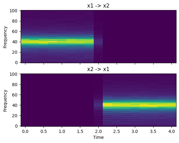
granger = c.pairwise_spectral_granger_prediction()

fig, ax = plt.subplots(2, 1, sharex=True, sharey=True)

ax[0].pcolormesh(
    c.time, c.frequencies, granger[..., :, 0, 1].T, cmap="viridis", shading="auto"
)
ax[0].set_title("x1 -> x2")
ax[0].set_ylabel("Frequency")
ax[1].pcolormesh(
    c.time, c.frequencies, granger[..., :, 1, 0].T, cmap="viridis", shading="auto"
)
ax[1].set_title("x2 -> x1")
ax[1].set_xlabel("Time")
ax[1].set_ylabel("Frequency")

/Users/edeno/miniconda3/envs/spectral_connectivity/lib/python3.7/site-packages/ipykernel_launcher.py:52: MatplotlibDeprecationWarning: shading='flat' when X and Y have the same dimensions as C is deprecated since 3.3.  Either specify the corners of the quadrilaterals with X and Y, or pass shading='auto', 'nearest' or 'gouraud', or set rcParams['pcolor.shading'].  This will become an error two minor releases later.
/Users/edeno/miniconda3/envs/spectral_connectivity/lib/python3.7/site-packages/ipykernel_launcher.py:55: MatplotlibDeprecationWarning: shading='flat' when X and Y have the same dimensions as C is deprecated since 3.3.  Either specify the corners of the quadrilaterals with X and Y, or pass shading='auto', 'nearest' or 'gouraud', or set rcParams['pcolor.shading'].  This will become an error two minor releases later.

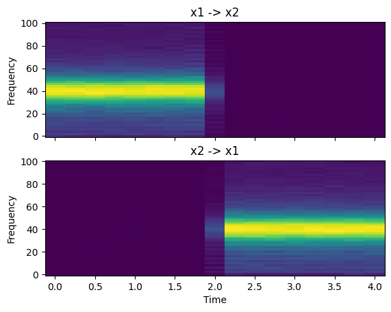
dtf = c.directed_transfer_function()

fig, ax = plt.subplots(2, 1, sharex=True, sharey=True)

ax[0].pcolormesh(
    c.time, c.frequencies, dtf[..., :, 0, 1].T, cmap="viridis", shading="auto"
)
ax[0].set_title("x1 -> x2")
ax[0].set_ylabel("Frequency")
ax[1].pcolormesh(
    c.time, c.frequencies, dtf[..., :, 1, 0].T, cmap="viridis", shading="auto"
)
ax[1].set_title("x2 -> x1")
ax[1].set_xlabel("Time")
ax[1].set_ylabel("Frequency")

/Users/edeno/miniconda3/envs/spectral_connectivity/lib/python3.7/site-packages/ipykernel_launcher.py:5: MatplotlibDeprecationWarning: shading='flat' when X and Y have the same dimensions as C is deprecated since 3.3.  Either specify the corners of the quadrilaterals with X and Y, or pass shading='auto', 'nearest' or 'gouraud', or set rcParams['pcolor.shading'].  This will become an error two minor releases later.
  """
/Users/edeno/miniconda3/envs/spectral_connectivity/lib/python3.7/site-packages/ipykernel_launcher.py:8: MatplotlibDeprecationWarning: shading='flat' when X and Y have the same dimensions as C is deprecated since 3.3.  Either specify the corners of the quadrilaterals with X and Y, or pass shading='auto', 'nearest' or 'gouraud', or set rcParams['pcolor.shading'].  This will become an error two minor releases later.
  

pdc = c.partial_directed_coherence()

fig, ax = plt.subplots(2, 1, sharex=True, sharey=True)

ax[0].pcolormesh(c.time, c.frequencies, pdc[..., :, 0, 1].T, cmap="viridis")
ax[0].set_title("x1 -> x2")
ax[0].set_ylabel("Frequency")
ax[1].pcolormesh(c.time, c.frequencies, pdc[..., :, 1, 0].T, cmap="viridis")
ax[1].set_title("x2 -> x1")
ax[1].set_xlabel("Time")
ax[1].set_ylabel("Frequency")

/Users/edeno/miniconda3/envs/spectral_connectivity/lib/python3.7/site-packages/ipykernel_launcher.py:5: MatplotlibDeprecationWarning: shading='flat' when X and Y have the same dimensions as C is deprecated since 3.3.  Either specify the corners of the quadrilaterals with X and Y, or pass shading='auto', 'nearest' or 'gouraud', or set rcParams['pcolor.shading'].  This will become an error two minor releases later.
  """
/Users/edeno/miniconda3/envs/spectral_connectivity/lib/python3.7/site-packages/ipykernel_launcher.py:8: MatplotlibDeprecationWarning: shading='flat' when X and Y have the same dimensions as C is deprecated since 3.3.  Either specify the corners of the quadrilaterals with X and Y, or pass shading='auto', 'nearest' or 'gouraud', or set rcParams['pcolor.shading'].  This will become an error two minor releases later.