Tutorial#
The spectral_connectivity package has two main classes used for computation:
MultitaperConnectivity.
There is also a function called multitaper_connectivity which combines the usage of the two classes and outputs a labeled array, which can be convenient for understanding the output and plotting.
This tutorial will walk you through the usage of each.
Multitaper#
Multitaper is used to compute the multitaper Fourier transform of a set of signals. It returns Fourier coefficients that can subsequently be used by the Connectivity class to compute frequency-domain metrics on the signals such as power and coherence.
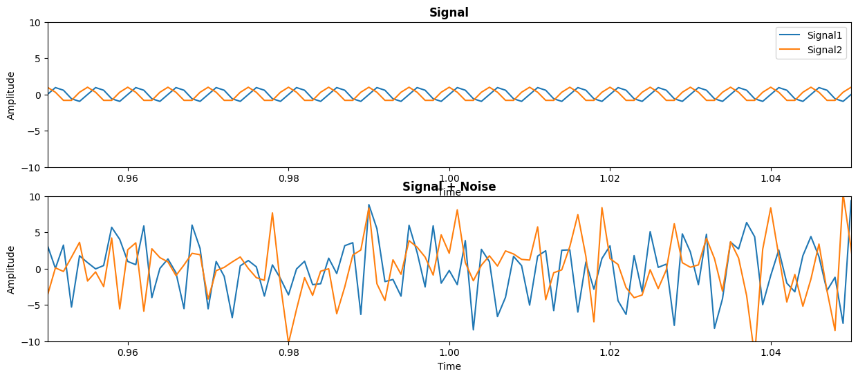
Let’s simulate a set of signals and see how to use the Multitaper class. We simulate two signals (signal) which oscillate at 200 Hz and are offset in phase by \(\frac{\pi}{2}\). We also simulate some white noise to add to the signal (noise). We want to compute the multitaper Fourier transform of these two signals.
import numpy as np

frequency_of_interest = 200
sampling_frequency = 1000
time_extent = (0, 60)
n_signals = 2


n_time_samples = ((time_extent[1] - time_extent[0]) * sampling_frequency) + 1

# Signal 1
time = np.linspace(time_extent[0], time_extent[1], num=n_time_samples, endpoint=True)
signal = np.zeros((n_time_samples, n_signals))
signal[:, 0] = np.sin(2 * np.pi * time * frequency_of_interest)

# Signal 2
phase_offset = np.pi / 2
signal[:, 1] = np.sin((2 * np.pi * time * frequency_of_interest) + phase_offset)

noise = np.random.normal(0, 4, signal.shape)
We can plot these two signals with and without the noise added:
import matplotlib.pyplot as plt

fig, axes = plt.subplots(2, 1, figsize=(15, 6))
axes[0].set_title("Signal", fontweight="bold")
axes[0].plot(time, signal[:, 0], label="Signal1")
axes[0].plot(time, signal[:, 1], label="Signal2")
axes[0].set_xlabel("Time")
axes[0].set_ylabel("Amplitude")
axes[0].set_xlim((0.95, 1.05))
axes[0].set_ylim((-10, 10))
axes[0].legend()

axes[1].set_title("Signal + Noise", fontweight="bold")
axes[1].plot(time, signal + noise)
axes[1].set_xlabel("Time")
axes[1].set_ylabel("Amplitude")
axes[1].set_xlim((0.95, 1.05))
axes[1].set_ylim((-10, 10))
(-10.0, 10.0)
Now let’s import the Multitaper class and see how to use it. From the docstring, we can see there are a number of inputs to the class. We will walk through the most important of these inputs.
from spectral_connectivity import Multitaper
from spectral_connectivity.transforms import prepare_time_series

?Multitaper
Init signature:
Multitaper(
    time_series: numpy.ndarray[tuple[typing.Any, ...], numpy.dtype[numpy.floating]],
    sampling_frequency: float = 1000,
    time_halfbandwidth_product: float = 3,
    detrend_type: str | None = 'constant',
    time_window_duration: float | None = None,
    time_window_step: float | None = None,
    n_tapers: int | None = None,
    tapers: numpy.ndarray[tuple[typing.Any, ...], numpy.dtype[numpy.floating]] | None = None,
    start_time: float | numpy.ndarray[tuple[typing.Any, ...], numpy.dtype[numpy.floating]] = 0,
    n_fft_samples: int | None = None,
    n_time_samples_per_window: int | None = None,
    n_time_samples_per_step: int | None = None,
    is_low_bias: bool = True,
) -> None
Docstring:
Multitaper spectral analysis for robust power spectral density estimation.

Transforms time-domain signals to frequency domain using multiple orthogonal
tapering windows (Slepian sequences). This approach reduces spectral leakage
and provides better spectral estimates than single-taper methods.

Parameters
----------
time_series : NDArray[floating], shape (n_time_samples, n_trials, n_signals)
    Input time series data. **Must be 3D array.**
    - n_time_samples: number of time points
    - n_trials: number of trials (use 1 for single trial)
    - n_signals: number of signals/channels
    Multiple trials are averaged in the spectral domain.

    **Important:** If your data is 1D or 2D, use `prepare_time_series()`
    helper function to convert it to the required 3D format.
sampling_frequency : float, default=1000
    Sampling rate in Hz of the time series data.
time_halfbandwidth_product : float, default=3
    Time-bandwidth product (often denoted as NW) controlling the trade-off
    between frequency resolution and variance reduction.

    **Effect on analysis:**
    - Determines frequency resolution: Δf = 2·NW / T (where T is window duration)
    - Determines number of tapers: n_tapers = floor(2·NW) - 1
    - Higher values → More spectral smoothing, better variance reduction
    - Lower values → Better frequency resolution, less averaging

    **Typical values:**
    - NW = 2: Minimal smoothing, 3 tapers, best frequency resolution
    - NW = 3: Balanced trade-off (recommended default), 5 tapers
    - NW = 4: More smoothing, 7 tapers, strong variance reduction
    - NW = 5+: Heavy smoothing, 9+ tapers, very strong variance reduction

    **Examples:**
    For 1 Hz frequency resolution with 1 second windows: use NW ≤ 0.5
    For 5 Hz frequency resolution with 1 second windows: use NW ≤ 2.5
    For 10 Hz frequency resolution with 1 second windows: use NW ≤ 5

    Use `estimate_frequency_resolution()` to calculate the resolution
    for different parameter combinations, or use `suggest_parameters()`
    to get recommendations for your specific data and analysis goals.
detrend_type : {"constant", "linear", None}, default="constant"
    Type of detrending applied to each time window:
    - "constant": remove DC component
    - "linear": remove linear trend
    - None: no detrending
time_window_duration : float, optional
    Duration in seconds of sliding time windows. If None, analyzes entire
    time series (no time resolution).
time_window_step : float, optional
    Step size in seconds between consecutive time windows. If None, uses
    non-overlapping windows (step = window duration).
n_tapers : int, optional
    Number of DPSS tapers to use. If None, computed as
    floor(2 * time_halfbandwidth_product) - 1.
tapers : NDArray[floating], shape (n_time_samples_per_window, n_tapers), optional
    Pre-computed tapering windows. If None, DPSS tapers are computed
    automatically.
start_time : float or NDArray[floating], default=0
    Start time in seconds of the time series data.
n_fft_samples : int, optional
    Length of FFT. If None, uses next power of 2 >= n_time_samples_per_window.
n_time_samples_per_window : int, optional
    Number of samples per time window. Computed from time_window_duration
    if not provided.
n_time_samples_per_step : int, optional
    Number of samples to advance between windows. Computed from
    time_window_step if not provided.
is_low_bias : bool, default=True
    If True, exclude tapers with eigenvalues < MIN_EIGENVALUE_THRESHOLD (0.9) to reduce bias.

Attributes
----------
fft : NDArray[complex128]
    Complex-valued FFT coefficients with shape
    (n_time_windows, n_trials, n_tapers, n_frequencies, n_signals).
frequencies : NDArray[float64], shape (n_frequencies,)
    Frequency values in Hz corresponding to FFT bins.
time : NDArray[float64], shape (n_time_windows,)
    Time values in seconds for center of each time window.

Examples
--------
Using the helper function (recommended for 2D data):

>>> import numpy as np
>>> from spectral_connectivity.transforms import Multitaper, prepare_time_series
>>> # EEG recording: 5 seconds at 1000 Hz, 64 channels
>>> eeg_data = np.random.randn(5000, 64)  # Shape: (n_time, n_channels)
>>> eeg_3d = prepare_time_series(eeg_data, axis='signals')
>>> mt = Multitaper(eeg_3d, sampling_frequency=1000, time_halfbandwidth_product=4)
>>> print(f"FFT shape: {mt.fft().shape}")
>>> print(f"Frequencies: {len(mt.frequencies)} bins, max = {mt.frequencies[-1]:.1f} Hz")

Manual reshaping with np.newaxis (advanced):

>>> # Generate test signal: 50Hz + noise
>>> fs = 1000  # 1 kHz sampling
>>> t = np.arange(0, 1, 1/fs)
>>> signal = np.sin(2*np.pi*50*t) + 0.1*np.random.randn(len(t))
>>> # Manually reshape to 3D: (n_time, n_trials, n_signals)
>>> data = signal[:, np.newaxis, np.newaxis]  # Shape: (1000, 1, 1)
>>> mt = Multitaper(data, sampling_frequency=fs, time_halfbandwidth_product=4)

Multiple trials (already 3D):

>>> # Epoched data: 100 trials, 5 channels, 1 second each at 1000 Hz
>>> epoched_data = np.random.randn(1000, 100, 5)  # (n_time, n_trials, n_signals)
>>> mt = Multitaper(epoched_data, sampling_frequency=1000)
>>> print(f"Trials: {mt.n_trials}, Signals: {mt.n_signals}")  # Trials: 100, Signals: 5

Notes
-----
The multitaper method uses discrete prolate spheroidal sequences (DPSS)
as tapers, which are optimal for spectral analysis in the sense of minimizing
spectral leakage while maximizing energy concentration in the frequency band
of interest.

References
----------
.. [1] Thomson, D. J. (1982). Spectrum estimation and harmonic analysis.
       Proceedings of the IEEE, 70(9), 1055-1096.
.. [2] Percival, D. B., & Walden, A. T. (1993). Spectral Analysis for
       Physical Applications. Cambridge University Press.
File:           ~/Documents/GitHub/spectral_connectivity/spectral_connectivity/transforms.py
Type:           type
Subclasses:
time_series#
The most important input is time_series. This array is what gets transformed into the frequency domain. The order of dimensions of time_series are critical for how the data is processed. The array can either have two or three dimensions.
If the array has two dimensions, then dimension 1 is time and dimensions 2 is signals. This is how our simulated signal is arranged. We have 50001 samples in the time dimension and 2 signals:
signal.shape
(60001, 2)
If we have three dimensions, dimension 1 is time, dimension 2 is trials, and dimensions 3 is signals. It is important to know note that dimension 2 now has a different meaning in that it represents trials and not signals now. Dimension 3 is now the signals dimension. We will show an example of this later.
sampling_frequency#
The next most important input is the sampling_frequency. The sampling_frequency is the number of samples per time unit the signal(s) are recorded at. This is set by default to 1000 samples per second. If your signal is sampled at a different rate, this needs to be set. In our simulated signal, we have sampled time at 1000 samples per second:
sampling_frequency
1000
time_halfbandwidth_product#
The time_halfbandwidth_product controls the frequency resolution of the Fourier transformed signal. It is equal to the duration of the time window multiplied by the half of the frequency resolution desired (the so-called half bandwidth). Remember that the frequency resolution is the number of consecutive frequencies that can be distinguished. So 2 Hz frequency resolution (which has a 1 Hz half bandwidth) means that we can tell the difference between 9 Hz and 11 Hz, but not 10 Hz.
Setting this parameter will define the default number of tapers used in the transform (number of tapers = 2 * time_halfbandwidth_product - 1.).
It is outside the scope of this tutorial to fully explain multitaper analysis, but a good introduction can be found in the book: Case Studies in Neural Data Analysis.
time_window_duration and time_window_step#
The time_window_duration controls the duration of the segment of time the transformation is computed on. This is specified in seconds and automatically set to the entire length of the signal(s) if it is not specified. For example, if you want to compute a spectrogram, you need to set the time_window_duration to something smaller than the length of the signal(s). Note that setting this will affect the frequency resolution as it is part of the calculation of the time_halfbandwidth_product (see above).
The time_window_step control how far the time window is slid. By default, the time window is set to slide the length of the time_window_duration so that each time window is non-overlapping (approximately independent). Setting the step to smaller than the time window duration will make the time windows overlap, so they will be dependent.
Using Multitaper#
Now that we know some of the inputs to Multitaper, let’s see how to use it. We will give the class a noisy signal (signal + noise), the sampling frequency (sampling_frequency) which we used to simulate the signals and set the time_halfbandwidth_product to 5:
# Convert signal to 3D format (n_time_samples, n_trials, n_signals)
signal_with_noise = prepare_time_series(signal + noise, axis="signals")
multitaper = Multitaper(
    signal_with_noise,
    sampling_frequency=sampling_frequency,
    time_halfbandwidth_product=5,
)
multitaper
Multitaper(sampling_frequency=1000, time_halfbandwidth_product=5,
           time_window_duration=60.001, time_window_step=60.001,
           detrend_type='constant', start_time=0, n_tapers=9)
We can see that instantiating the class into the variable (multitaper) automatically computed some properties. For example, we can look at time_window_duration and time_window_step, which both will be the length of the entire signal because we did not specify a shorter duration:
multitaper.time_window_duration
60.001
multitaper.time_window_step
60.001
We can also look at the frequency resolution (which is determined by the time_halfbandwidth_product and the time_window_duration).
NOTE: The bandwidth is another way to refer to the frequency resolution.
multitaper.frequency_resolution
0.1666638889351844
We can also compute the nyquist frequency, which is the highest resolvable frequency. This is half the sampling frequency.
multitaper.nyquist_frequency
500.0
Note that we haven’t run the tranformation yet. To do this we can use the method fft to get the Fourier coefficients.
This will have shape (n_time_windows, n_trials, n_tapers, n_fft_samples, n_signals).
fourier_coefficients = multitaper.fft()
fourier_coefficients.shape
(1, 1, 9, 60025, 2)
We can get the time corresponding to each time window (of length n_time_windows) and the frequencies (of length n_fft_samples).
multitaper.time
array([0.])
multitaper.frequencies
array([ 0.        ,  0.01665973,  0.03331945, ..., -0.04997918,
       -0.03331945, -0.01665973], shape=(60025,))
In this case, we have computed the Fourier transform on the entire signal, so we only have a single time corresponding to the beginning of the time window (0.0).
Also note that the frequencies given by the Multitaper class are both positive and negative. This is necessary for certain computations.
Now that we have computed the fft we have all the ingredients we need to compute the connectivity measures.
The Connectivity class#
The Connectivity class computes the frequency-domain connectivity measures from the Fourier coeffcients. Let’s import the class and look at the docstring:
from spectral_connectivity import Connectivity

?Connectivity
Init signature:
Connectivity(
    fourier_coefficients: numpy.ndarray[tuple[typing.Any, ...], numpy.dtype[numpy.complexfloating]],
    expectation_type: str = 'trials_tapers',
    frequencies: numpy.ndarray[tuple[typing.Any, ...], numpy.dtype[numpy.floating]] | None = None,
    time: numpy.ndarray[tuple[typing.Any, ...], numpy.dtype[numpy.floating]] | None = None,
    blocks: int | None = None,
    dtype: numpy.dtype = <class 'numpy.complex128'>,
) -> None
Docstring:
Compute functional and directed connectivity measures from spectral data.

This class provides a comprehensive suite of connectivity analysis methods
based on cross-spectral matrices derived from Fourier-transformed time series.
Methods range from basic coherence to advanced Granger causality measures.

Parameters
----------
fourier_coefficients : NDArray[complexfloating],
    shape (n_time_windows, n_trials, n_tapers, n_frequencies, n_signals)
    Complex-valued Fourier coefficients from spectral analysis. Must be
    two-sided (positive and negative frequencies) for Granger methods.
    Usually obtained from multitaper or other spectral estimation methods.
    **Validation**: Must be 5-dimensional with at least 2 signals and
    contain only finite values (no NaN/Inf).
expectation_type : {"trials_tapers", "trials", "tapers", "time",
    "time_trials", "time_tapers", "time_trials_tapers"},
    default="trials_tapers"
    Specifies how to average the cross-spectral matrix:
    - "trials_tapers": average over trials and tapers (most common)
    - "trials": average over trials only (keep taper dimension)
    - "tapers": average over tapers only (keep trial dimension)
    - "time": average over time windows
    - combinations: average over multiple dimensions
frequencies : NDArray[floating], shape (n_frequencies,), optional
    Frequency values in Hz corresponding to FFT bins. If None, uses
    normalized frequencies.
time : NDArray[floating], shape (n_time_windows,), optional
    Time values in seconds for each time window. If None, uses indices.
blocks : int, optional
    Number of blocks for memory-efficient computation of large connectivity
    matrices. When specified, the cross-spectral matrix is computed in
    chunks rather than all at once, reducing peak memory usage.

    **When to use blocks:**

    - Large number of signals (n_signals >= 50, as a rough guideline;
      benefit increases with more signals)
    - Memory-constrained environments
    - High-resolution spectrograms (large n_time_windows × n_frequencies)
    - GPU computing with limited VRAM

    **When NOT to use blocks:**

    - Small datasets (n_signals < 50): The overhead of block management
      may exceed the memory benefit, making blocks=None faster
    - When speed is critical and memory is abundant

    **Memory-Speed Tradeoff:**

    - **Without blocks** (default): Fastest for small datasets, but requires
      memory for full (n_time_windows × n_frequencies × n_signals × n_signals)
      array
    - **With blocks**: Reduces peak memory by 70-80% for large arrays
      (measured 73% reduction for n_signals=50, blocks=5), with minimal
      speed penalty (typically <10%)

    **Quick Decision Guide:**

    - n_signals < 50: Use default (blocks=None)
    - 50 ≤ n_signals < 100: Use blocks=5 if memory is limited
    - n_signals ≥ 100: Recommended blocks=5 or blocks=10
    - Out of memory errors: Increase blocks value (try doubling)

    **Important**: Results are numerically identical whether using blocks
    or not (validated to floating-point precision).
dtype : np.dtype, default=complex128
    Data type for internal computations. Should match input precision.

Attributes
----------
n_observations : int
    Effective number of independent observations after averaging,
    used for statistical inference.

Examples
--------
>>> import numpy as np
>>> from spectral_connectivity import Connectivity
>>> # Simulate coherent signals
>>> n_times, n_trials, n_tapers, n_freqs, n_signals = 50, 10, 5, 100, 2
>>> # Create complex coefficients with some coherence
>>> phase_diff = np.pi/4  # 45 degree phase difference
>>> coeffs = np.random.randn(n_times, n_trials, n_tapers, n_freqs, n_signals) +     ...          1j * np.random.randn(n_times, n_trials, n_tapers, n_freqs, n_signals)
>>> # Add coherence at specific frequencies
>>> coeffs[:, :, :, 10, 1] = coeffs[:, :, :, 10, 0] * np.exp(1j * phase_diff)
>>>
>>> # Compute connectivity
>>> conn = Connectivity(coeffs, expectation_type="trials_tapers")
>>> coherence = conn.coherence_magnitude()  # Shape: (n_times, n_freqs, 2, 2)
>>> phase_lag = conn.coherence_phase()
>>> print(f"Coherence shape: {coherence.shape}")
>>> print(f"Peak coherence: {np.max(coherence[:, 10, 0, 1]):.3f}")

Notes
-----
The class supports both CPU (NumPy) and GPU (CuPy) computation depending
on the SPECTRAL_CONNECTIVITY_ENABLE_GPU environment variable. For Granger
causality measures, minimum phase decomposition [1]_ is used to estimate
transfer functions and noise covariances non-parametrically.

References
----------
.. [1] Dhamala, M., Rangarajan, G., and Ding, M. (2008). Analyzing
       information flow in brain networks with nonparametric Granger
       causality. NeuroImage 41, 354-362.
.. [2] Bastos, A. M., & Schoffelen, J. M. (2016). A tutorial review of
       functional connectivity analysis methods and their interpretational
       pitfalls. Frontiers in systems neuroscience, 9, 175.
File:           ~/Documents/GitHub/spectral_connectivity/spectral_connectivity/connectivity.py
Type:           type
Subclasses:
From the docstring, we can see that the Connectivity class is initialized with the following parameters:
fourier_coefficientsexpectation_typefrequencies,timeblocksdtype
Of these, we have already computed the fourier_coefficients, time, and frequencies from the Multitaper class (see last section). We will consider the most important remaining parameters in turn:
expectation_type#
The expectation_type is perhaps the most important of the parameters to consider. It defines the dimensions of the cross-spectrum that are averaged over. You can average over any combination of:
time
trials
tapers
By default, Connectivity averages over trials and tapers (trials_tapers), but depending on your usage, you may want to average over the other dimensions. The dimensions you average over is specified by a string with an underscore (_) between the dimensions.
Note that the order of the dimensions must be in the order time, trials, and tapers. So if you wish to average over all three, the correct expectation type is time_trials_tapers and not trials_time_tapers.
blocks#
The blocks parameter can help when the computation of the connectivity measures is taking up a large amount of RAM. The computation of the cross-spectral matrix can be large depending on the number of time samples, frequencies, trials and tapers. Therefore it is sometimes useful to simplify this by breaking this computation up into smaller arrays (blocks). The blocks parameter controls the number of blocks the matrix is split into. Setting this parameter appropriately is a matter of experimentation, but users should start with the default of 1 and increase it as needed as memory usage becomes a problem.
Using Connectivity#
Okay, now that we understand the parameters, we can now instantiate the class in order to compute the connectivity measures. You can instantiate the class as follows:
connectivity = Connectivity(
    fourier_coefficients=multitaper.fft(),
    expectation_type="trials_tapers",
    frequencies=multitaper.frequencies,
    time=multitaper.time,
    blocks=1,
)
Alternatively, you can also instantiate the class this way, which is a little more convenient code-wise. Note that in this formulation, you do not call the .fft method, the class method from_multitaper does this for you:
connectivity = Connectivity.from_multitaper(multitaper)
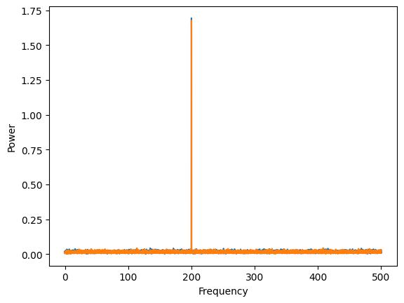
We are now ready to compute the connectivity measures. These all exists as function methods on the class. So for instance, if you want to compute the power of the two signals, we would use the power method:
power = connectivity.power()
power.shape
(1, 30013, 2)
Notice here that only the non-negative frequencies are returned (since for real signals, the power spectrum is symmetric). Also since we didn’t average over time (the expectation_type is “trials_tapers” by default), it is included in the first dimension. We can get the non-negative frequencies using the frequencies property. Notice that the shape of the second dimension of power matches:
connectivity.frequencies.shape
(30013,)
We could also average over time here since there is only one time point – the average will have no effect other than to remove the time dimension from the output. Let’s try that here:
connectivity = Connectivity.from_multitaper(
    multitaper, expectation_type="time_trials_tapers", blocks=1
)
connectivity.power().shape
(30013, 2)
Let’s plot the power of both signals. Remember that we simulated them both to be 200 Hz oscillations, offset by \(\frac{\pi}{2}\) in phase. As expected, the power of both signals is at 200 Hz.
plt.plot(connectivity.frequencies, connectivity.power())
plt.ylabel("Power")
plt.xlabel("Frequency")
Text(0.5, 0, 'Frequency')
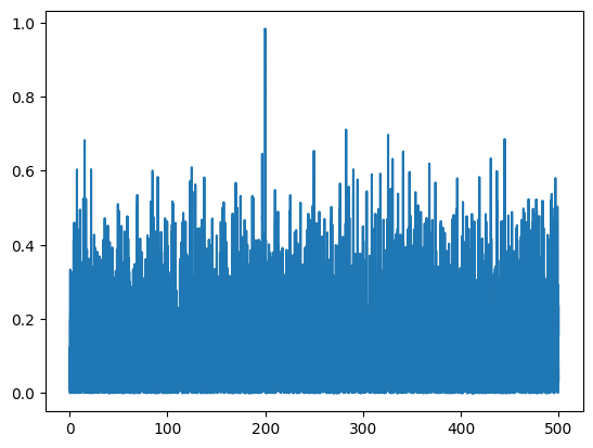
Now let’s say we want to compute the coherence, a measure of how stable the phase relationships are between the two signals. We use the coherence_magnitude method to compute this.
coherence = connectivity.coherence_magnitude()
coherence.shape
(30013, 2, 2)
The coherence comes in shape (n_frequencies, n_signals, n_signals). Because it is symmetric, we only have to plot the relationship from signal1 to signal2. We can see that the signal is more coherent at 200 Hz.
plt.plot(connectivity.frequencies, coherence[:, 0, 1])
[<matplotlib.lines.Line2D at 0x2a5429070>]
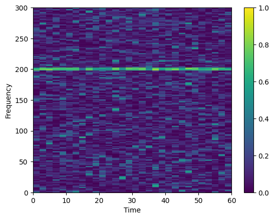
Adding in time#
Suppose we want to look at how coherence evolves over time. To do so, we have to go back to the Multitaper class and specify the time_window_duration. Here we set it to be 2 seconds. Then we can compute the coherence again from the Connectivity class.
multitaper = Multitaper(
    signal_with_noise,
    sampling_frequency=sampling_frequency,
    time_halfbandwidth_product=5,
    time_window_duration=2.0,
)
connectivity = Connectivity.from_multitaper(
    multitaper, expectation_type="trials_tapers"
)

coherence = connectivity.coherence_magnitude()
coherence.shape
(30, 1001, 2, 2)
Also note how this changes our frequency resolution.
multitaper.frequency_resolution
5.0
Now we can plot the coherence over time
time_grid, freq_grid = np.meshgrid(
    np.append(connectivity.time, time_extent[-1]),
    np.append(connectivity.frequencies, multitaper.nyquist_frequency),
)

mesh = plt.pcolormesh(
    time_grid,
    freq_grid,
    connectivity.coherence_magnitude()[..., 0, 1].squeeze().T,
    vmin=0.0,
    vmax=1.0,
    cmap="viridis",
)
plt.ylim((0, 300))
plt.xlim(time_extent)
plt.xlabel("Time")
plt.ylabel("Frequency")
plt.colorbar()
<matplotlib.colorbar.Colorbar at 0x2a114d3a0>
There are a number of other connectivity measures besides coherence. See the other notebooks for examples on how to use them.
multitaper_connectivity#
There is a third option for how to compute the connectivity measures. The output of this option is a labeled array using the xarray package. This can be convenient because one always knows what the dimensions are. In addition, xarray arrays make plotting easy.
Let’s repeat the example above of computing the coherence over time with this interface and see how this makes things easier.
from spectral_connectivity import multitaper_connectivity

coherence = multitaper_connectivity(
    signal_with_noise,
    sampling_frequency=sampling_frequency,
    time_halfbandwidth_product=5,
    time_window_duration=2.0,
    method="coherence_magnitude",
)

coherence
<xarray.DataArray 'coherence_magnitude' (time: 30, frequency: 1001, source: 2,
                                         target: 2)> Size: 961kB
array([[[[       nan, 0.45918036],
         [0.45918036,        nan]],

        [[       nan, 0.25961805],
         [0.25961805,        nan]],

        [[       nan, 0.34489352],
         [0.34489352,        nan]],

        ...,

        [[       nan, 0.15043708],
         [0.15043708,        nan]],

        [[       nan, 0.2058857 ],
         [0.2058857 ,        nan]],

        [[       nan, 0.18139946],
         [0.18139946,        nan]]],

...

       [[[       nan, 0.00740096],
         [0.00740096,        nan]],

        [[       nan, 0.01180062],
         [0.01180062,        nan]],

        [[       nan, 0.07439174],
         [0.07439174,        nan]],

        ...,

        [[       nan, 0.15354869],
         [0.15354869,        nan]],

        [[       nan, 0.00108677],
         [0.00108677,        nan]],

        [[       nan, 0.00625096],
         [0.00625096,        nan]]]], shape=(30, 1001, 2, 2))
Coordinates:
  * time       (time) float64 240B 0.0 2.0 4.0 6.0 8.0 ... 52.0 54.0 56.0 58.0
  * frequency  (frequency) float64 8kB 0.0 0.5 1.0 1.5 ... 499.0 499.5 500.0
  * source     (source) <U1 8B '0' '1'
  * target     (target) <U1 8B '0' '1'
Attributes: (12/16)
    mt_detrend_type:                constant
    mt_frequency_resolution:        5.0
    mt_is_low_bias:                 True
    mt_n_fft_samples:               2000
    mt_n_signals:                   2
    mt_n_tapers:                    9
    ...                             ...
    mt_sampling_frequency:          1000
    mt_start_time:                  0
    mt_summarize_parameters:        <bound method Multitaper.summarize_parame...
    mt_time_halfbandwidth_product:  5
    mt_time_window_duration:        2.0
mt_time_window_step: 2.0We see that the labeled output conveniently gives us the time and frequencies and signal labels for each dimension. Manipulating xarray by their label name is convenient. Lets’ say we only want frequencies between 100 and 300 Hz. We can grab this data in a convenient way:
coherence.sel(frequency=slice(100, 300))
<xarray.DataArray 'coherence_magnitude' (time: 30, frequency: 401, source: 2,
                                         target: 2)> Size: 385kB
array([[[[       nan, 0.09630359],
         [0.09630359,        nan]],

        [[       nan, 0.06003863],
         [0.06003863,        nan]],

        [[       nan, 0.08824564],
         [0.08824564,        nan]],

        ...,

        [[       nan, 0.06787789],
         [0.06787789,        nan]],

        [[       nan, 0.04864566],
         [0.04864566,        nan]],

        [[       nan, 0.03176439],
         [0.03176439,        nan]]],

...

       [[[       nan, 0.04377205],
         [0.04377205,        nan]],

        [[       nan, 0.03295512],
         [0.03295512,        nan]],

        [[       nan, 0.04093662],
         [0.04093662,        nan]],

        ...,

        [[       nan, 0.02097841],
         [0.02097841,        nan]],

        [[       nan, 0.0131043 ],
         [0.0131043 ,        nan]],

        [[       nan, 0.07531392],
         [0.07531392,        nan]]]], shape=(30, 401, 2, 2))
Coordinates:
  * time       (time) float64 240B 0.0 2.0 4.0 6.0 8.0 ... 52.0 54.0 56.0 58.0
  * frequency  (frequency) float64 3kB 100.0 100.5 101.0 ... 299.0 299.5 300.0
  * source     (source) <U1 8B '0' '1'
  * target     (target) <U1 8B '0' '1'
Attributes: (12/16)
    mt_detrend_type:                constant
    mt_frequency_resolution:        5.0
    mt_is_low_bias:                 True
    mt_n_fft_samples:               2000
    mt_n_signals:                   2
    mt_n_tapers:                    9
    ...                             ...
    mt_sampling_frequency:          1000
    mt_start_time:                  0
    mt_summarize_parameters:        <bound method Multitaper.summarize_parame...
    mt_time_halfbandwidth_product:  5
    mt_time_window_duration:        2.0
mt_time_window_step: 2.0We can also plot this in an easy way that puts the labels on the plot:
coherence.sel(frequency=slice(100, 300)).plot(
    x="time", y="frequency", row="source", col="target"
)
<xarray.plot.facetgrid.FacetGrid at 0x2a54dd730>
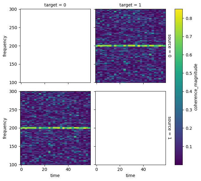
Fully explaining using xarray arrays is beyond the scope of this tutorial, but see the xarray documentation to explore all the possibilities.
Using GPUs#
The spectral_connectivity package can do computations on the GPU to speed up the code. To do this, you must have the package cupy installed AND have the environmental variable SPECTRAL_CONNECTIVITY_ENABLE_GPU set.
WARNING: the environmental variable must be set before the first import of the spectral_connectivity package or the GPU enabled functions will not work.
To check if you are using the GPU on first import, use the logging.basicConfig to get messages that will tell you which version is being used.
It is easiest to use conda to install cupy because it handles the installation of the correct version of cudatoolkit. Note that cupy will not work on Macs.